Leveraging SIMD in Rust for High-Performance Computing
Learn how to use SIMD in Rust to accelerate computations using both safe abstractions and low-level intrinsics for high-performance applications.

Daniel Gustaw
• 13 min read

Introduction
Rust gives you the power of low-level control with memory safety. Using SIMD (single instruction, multiple data), you can vectorize computations to process multiple data points at once, making tasks like numerical computing, graphics, or AI faster.
SIMD in Rust: Overview
Rust provides SIMD support in two main ways:
-
SIMD via
std::simd(introduced in Rust 1.70+):- Provides portable, safe SIMD abstractions.
- Works across different architectures.
- Vector types:
Simd<T, N>whereTis the scalar type andNis the number of lanes.
-
Low-level intrinsics (via
core::arch):- Unsafe, but gives full control over CPU instructions (e.g., SSE, AVX).
- Useful for performance-critical code.
Example 1: Hello world using std::simd
There is not enough of code using SIMD created by our civilization, so LLMs are bad at generating it.
Here is a simple example of adding two vectors using std::simd:
#![feature(portable_simd)]
use std::simd::Simd;

fn main() {
    // Hardcoded "random" single-digit numbers
    let a = Simd::<f32, 8>::from_array([3.0, 5.0, 1.0, 4.0, 2.0, 1.0, 8.0, 0.0]);
    let b = Simd::<f32, 8>::from_array([6.0, 2.0, 4.0, 2.0, 7.0, 3.0, 0.0, 5.0]);
    // SIMD addition
    let result = a + b;

    println!("Vector a: {:?}", a);
    println!("Vector b: {:?}", b);
    println!("Result: {:?}", result);
}
If we just run this code, it will fail with the following error:
error[E0554]: `#![feature]` may not be used on the stable release channel
 --> src/lib.rs:2:1
  |
2 | #![feature(portable_simd)]
we can
run it with the nightly compiler:
cargo +nightly runor even better set toolchain in file rust-toolchain.toml
[toolchain]
channel = "nightly"
this file not only saves us time for typing +nightly to every command but also help for IDE to recognize nightly
features. As result, we should see:
Vector a: [3.0, 5.0, 1.0, 4.0, 2.0, 1.0, 8.0, 0.0]
Vector b: [6.0, 2.0, 4.0, 2.0, 7.0, 3.0, 0.0, 5.0]
Result: [9.0, 7.0, 5.0, 6.0, 9.0, 4.0, 8.0, 5.0]
Example 2: Using core::arch Intrinsics (Unsafe SIMD)
#[cfg(target_arch = "x86_64")]
use core::arch::x86_64::*;

fn main() {
    unsafe {
        let a = _mm_set_ps(1.0, 5.0, 3.0, 2.0); // 128-bit register
        let b = _mm_set_ps(4.0, 3.0, 5.0, 1.0);
        let result = _mm_add_ps(a, b);

        let mut out = [0.0f32; 4];
        _mm_storeu_ps(out.as_mut_ptr(), result);

        println!("Vector a: {:?}", a);
        println!("Vector b: {:?}", b);
        println!("Result: {:?}", out);
    }
}
For these instructions you do not need +nightly flag or rust-toolchain.toml file.
It works perfectly on modern x86_64 cpus printing output:
Vector a: __m128(2.0, 3.0, 5.0, 1.0)
Vector b: __m128(1.0, 5.0, 3.0, 4.0)
Result: [3.0, 8.0, 8.0, 5.0]
but on other architectures (like ARM) it will fail with:
error[E0425]: cannot find function `_mm_set_ps` in this scope
 --> src/bin/core.rs:6:17
  |
6 |         let a = _mm_set_ps(1.0, 2.0, 3.0, 4.0); // 128-bit register
  |                 ^^^^^^^^^^ not found in this scope
For example, for Mac M1 your program should use NEON instead of SSE and look like this:
#[cfg(target_arch = "aarch64")]
use core::arch::aarch64::*;

fn main() {
    unsafe {
        let a = vld1q_f32([1.0,2.0,5.0,8.0].as_ptr());
        let b = vld1q_f32([7.0,3.0,1.0,0.0].as_ptr());
        let result = vaddq_f32(a, b);

        let mut out = [0.0f32; 4];
        vst1q_f32(out.as_mut_ptr(), result);

        println!("Vector a: {:?}", a);
        println!("Vector b: {:?}", b);
        println!("Result {:?}", out);
    }
}
On Mac (M series) it will print:
Vector a: float32x4_t(1.0, 2.0, 5.0, 8.0)
Vector b: float32x4_t(7.0, 3.0, 1.0, 0.0)
Result [8.0, 5.0, 6.0, 8.0]
but on x86_64 processors it will fail.
SIMD Instruction Set Extensions: SSE, AVX, NEON
Focusing on quick, practical intro, I mentioned a few terms:
- SSE (Streaming SIMD Extensions)
- AVX (Advanced Vector Extensions)
- NEON
Let’s look at them closer:
What they are
SSE, AVX, and NEON are SIMD instruction set extensions.
They are not separate architectures or protocols, but specialized sets of CPU instructions that extend a processor’s
base instruction set to support vectorized (parallel) operations.
In other words:
- They define how a CPU can operate on multiple pieces of data at once.
- They are part of the processor’s ISA (Instruction Set Architecture), not separate standards like networking protocols.
SSE (Streaming SIMD Extensions)
- Vendor: Intel (also supported by AMD).
- Introduced: 1999, with Pentium III.
- Registers: 128-bit (
XMM). - Capabilities:
- Process 4 ×
f32(floats) or 2 ×f64(doubles) simultaneously. - Widely used for multimedia, graphics, audio, and scientific workloads.
- Process 4 ×
- Successors: SSE2, SSE3, SSE4 (progressive improvements).
AVX (Advanced Vector Extensions)
- Vendor: Intel & AMD.
- Introduced: 2011, with Sandy Bridge CPUs.
- Registers:
- 256-bit (
YMM) in AVX/AVX2. - 512-bit (
ZMM) in AVX-512.
- 256-bit (
- Capabilities:
- Process 8 ×
f32or 4 ×f64(AVX-256). - Process 16 ×
f32or 8 ×f64(AVX-512).
- Process 8 ×
- Key points:
- Much higher throughput than SSE.
- More power-hungry; sometimes downclocked under a heavy load.
NEON
- Vendor: ARM (standard in ARMv7 and ARMv8).
- Introduced: 2009, with the ARMv7-A architecture.
- Registers: 128-bit (
Qregisters). - Capabilities:
- 4 ×
f32or 2 ×f64. - 8 ×
i16, 16 ×i8, etc.
- 4 ×
- Key points:
- ARM’s equivalent to SSE/AVX.
- Found in mobile processors and Apple Silicon (M1, M2, M3).
- Optimized for multimedia, AI, and signal processing workloads.
Summary Table
| Extension | Vendor | Register Width | Example Ops |
|---|---|---|---|
| SSE | Intel/AMD | 128-bit | 4×f32 add, 2×f64 mul |
| AVX | Intel/AMD | 256-bit / 512-bit | 8–16×f32, 4–8×f64 |
| NEON | ARM | 128-bit | 4×f32 add, 2×f64 mul |
Conclusion
- SSE and AVX are Intel/AMD SIMD instruction set extensions.
- NEON is ARM’s SIMD extension.
- All three are part of the CPU’s instruction set architecture (ISA).
- They serve the same purpose: speeding up data-parallel workloads like graphics, multimedia, scientific computing, and AI.
You can check support for these instructions of your CPU by commands like
lscpu | grep -i sse
lscpu | grep -i avx
Benchmarking
But hello world is not enough to show the power of SIMD. To see them in action, we have to compare the performance of
SIMD and no SIMD code.
We will use criterion crate for benchmarking.
Let’s start from creation of function that will add two arrays in src/lib.rs:
If SIMD would not exist we could write code like this:
pub fn add_arrays_fallback(a: &[f32], b: &[f32], out: &mut [f32]) {
    assert_eq!(a.len(), b.len(), "Input slices must have the same length");
    assert_eq!(a.len(), out.len(), "Output slice must match input length");

    // Scalar fallback
    for i in 0..a.len() {
        out[i] = a[i] + b[i];
    }
}
instead of fn(a,b) -> out, we are applying convention fn(a,b, mut out) -> void to save memory movements.
This function is quite clear. We iterate over all elements of a and b and add them to proper out slots.
For SIMD we have to group our data into chunks of 8 floats and then apply SIMD instruction. Finally, use fallback
method for leftovers.
#![feature(portable_simd)]

use itertools::izip;
use std::simd::f32x8;

pub fn add_arrays_simd(a: &[f32], b: &[f32], out: &mut [f32]) {
    assert_eq!(a.len(), b.len(), "Input slices must have the same length");
    assert_eq!(a.len(), out.len(), "Output slice must match input length");

    let lanes = f32x8::LEN; // 8 elements at once
    for (chunk_a, chunk_b, chunk_out) in izip!(
        a.chunks_exact(lanes),
        b.chunks_exact(lanes),
        out.chunks_exact_mut(lanes)
    ) {
        let va = f32x8::from_slice(chunk_a) + f32x8::from_slice(chunk_b);

        va.copy_to_slice(chunk_out);
    }

    // handle leftovers
    let remainder = a.len() % lanes;
    if remainder > 0 {
        let start = a.len() - remainder;
        for i in 0..remainder {
            out[start + i] = a[start + i] + b[start + i];
        }
    }
}
to simplify iteration over groups of 8 elements, we use itertools crate so we need to add to Cargo.toml:
[dependencies]
itertools = "0.14.0"
To install criterion crate, we should add also:
[dev-dependencies]
criterion = "0.7.0"

[[bench]]
name = "add_arrays_bench"
harness = false
and create file benches/add_arrays_bench.rs with content:
use criterion::{ criterion_group, criterion_main, Criterion };
use std::hint::black_box;
use simd_hello_world::{ add_arrays_simd, add_arrays_fallback };

fn big_arrays() -> (Vec<f32>, Vec<f32>, Vec<f32>) {
    let n = 10_000_000; // 10M elements
    let a: Vec<f32> = (0..n).map(|i| (i as f32) * 0.5).collect();
    let b: Vec<f32> = (0..n).map(|i| (i as f32) * 1.5).collect();
    let out = vec![0.0; n];
    (a, b, out)
}

fn bench_add_arrays(c: &mut Criterion) {
    let (a, b, mut out) = big_arrays();

    c.bench_function("add_arrays SIMD=true (10M)", |bench| {
        bench.iter(|| {
            add_arrays_simd(black_box(&a), black_box(&b), black_box(&mut out));
        });
    });

    c.bench_function("add_arrays SIMD=false (10M)", |bench| {
        bench.iter(|| {
            add_arrays_fallback(black_box(&a), black_box(&b), black_box(&mut out));
        });
    });
}

criterion_group!(benches, bench_add_arrays);
criterion_main!(benches);
Now typing
cargo benchwe will see
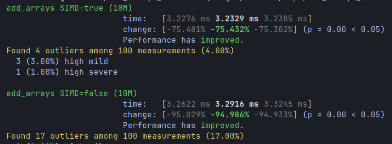
When I saw this result for the first time, I was highly disappointed.
Execution time 3.2329 ms and 3.2916 ms are nearly the same, while implementation complexity of add_arrays_simd is
much higher than old good add_arrays_fallback.
The reason for such a weak result of SIMD is in the fact that SIMD main constraint is pushing data from RAM to
CPU. Addition is such a quick and optimized operation that it nearly not takes time, so we’re spending all time of
benchmark to send data between RAM and CPU. In both cases there is the same amount of data, and parallelization of
superfast addition does not have any impact.
To see the difference, we have to add more complexity to computations, allowing our program to spend more time waiting for CPU than
moving data. It could be for example: a[i] = sqrt(a[i]) + log(b[i]), but we will use parametrized method
for _ in 0..complexity {
    a = a * a + f32x8::splat(0.5);
}
where complexity is a parameter that we can increase. Our new functions will look like:
pub fn add_arrays_simd_with_complexity(a: &[f32], b: &[f32], out: &mut [f32], complexity: Option<usize>) {
    assert_eq!(a.len(), b.len(), "Input slices must have the same length");
    assert_eq!(a.len(), out.len(), "Output slice must match input length");

    let complexity = complexity.unwrap_or(0);

    let lanes = f32x8::LEN; // 8 elements at once
    for (chunk_a, chunk_b, chunk_out) in izip!(
        a.chunks_exact(lanes),
        b.chunks_exact(lanes),
        out.chunks_exact_mut(lanes)
    ) {
        let mut va = f32x8::from_slice(chunk_a) + f32x8::from_slice(chunk_b);

        for _ in 0..complexity {
            va = va * va + f32x8::splat(0.5);
        }

        va.copy_to_slice(chunk_out);
    }

    // handle leftovers
    let remainder = a.len() % lanes;
    if remainder > 0 {
        let start = a.len() - remainder;
        for i in 0..remainder {
            let mut val = a[start + i] + b[start + i];
            for _ in 0..complexity {
                val = val * val + 0.5;
            }
            out[start + i] = val;
        }
    }
}

pub fn add_arrays_fallback_with_complexity(a: &[f32], b: &[f32], out: &mut [f32], complexity: Option<usize>) {
    assert_eq!(a.len(), b.len(), "Input slices must have the same length");
    assert_eq!(a.len(), out.len(), "Output slice must match input length");

    let complexity = complexity.unwrap_or(0);

    // Scalar fallback
    for i in 0..a.len() {
        let mut val = a[i] + b[i];
        for _ in 0..complexity {
            val = val * val + 0.5;
        }
        out[i] = val;
    }
}
it is basically the same as earlier, but instead of just simple addition,
now we’re adding and elements and complexity times replacing by its square increased by 0.5.
We can adjust our bench to form
use criterion::{Criterion, criterion_group, criterion_main};
use simd_hello_world::{
    add_arrays_fallback_with_complexity,
    add_arrays_simd_with_complexity,
};
use std::hint::black_box;

fn big_arrays() -> (Vec<f32>, Vec<f32>, Vec<f32>) {
    let n = 10_000_000; // 10M elements
    let a: Vec<f32> = (0..n).map(|i| (i as f32) * 0.5).collect();
    let b: Vec<f32> = (0..n).map(|i| (i as f32) * 1.5).collect();
    let out = vec![0.0; n];
    (a, b, out)
}

fn bench_add_arrays(c: &mut Criterion) {
    let (a, b, mut out) = big_arrays();

    for comp in 0..40 {
        c.bench_function(format!("add_arrays SIMD=true (10M) complexity {}", comp).as_str(), |bench| {
            bench.iter(|| {
                add_arrays_simd_with_complexity(
                    black_box(&a),
                    black_box(&b),
                    black_box(&mut out),
                    Some(comp),
                );
            });
        });

        c.bench_function(format!("add_arrays SIMD=false (10M) complexity {}", comp).as_str(), |bench| {
            bench.iter(|| {
                add_arrays_fallback_with_complexity(
                    black_box(&a),
                    black_box(&b),
                    black_box(&mut out),
                    Some(comp),
                );
            });
        });
    }
}

criterion_group!(benches, bench_add_arrays);
criterion_main!(benches);
and run by:
cargo benchResults analysis
When we paste benchmark results to benchmark.txt and parse it by script
import re
import sys

def parse_benchmarks(log_text: str):
    data = []
    # Regex to capture SIMD, complexity and the three times (with or without "ms")
    pattern = re.compile(
        r"add_arrays SIMD=(true|false).*?complexity (\d+).*?time:\s+\[([0-9.]+)\s*ms\s+([0-9.]+)\s*ms\s+([0-9.]+)\s*ms\]",
        re.DOTALL
    )

    for match in pattern.finditer(log_text):
        simd_str, complexity, low, mean, high = match.groups()
        simd = 1 if simd_str == "true" else 0
        comp = int(complexity)
        mean_time = float(mean)  # clean number now
        data.append([comp, simd, mean_time])

    return data

if __name__ == "__main__":
    # usage: python parse.py benchmarks.txt
    text = open(sys.argv[1]).read()
    parsed = parse_benchmarks(text)
    print("[")
    for row in parsed:
        print(f"  {row},")
    print("]")
we will see array
[
  [0, 1, 3.2136],
  [0, 0, 3.1748],
  [1, 1, 3.2488],
  ...
]
We can visualize it by matplotlib:
import matplotlib.pyplot as plt
import numpy as np

# Data provided
data = [
  [0, 1, 3.2136],
  [0, 0, 3.1748],
  [1, 1, 3.2488],
  [1, 0, 4.6649],
  [2, 1, 3.2924],
  [2, 0, 6.1988],
  [3, 1, 3.3776],
  [3, 0, 7.6825],
  [4, 1, 3.3826],
  [4, 0, 9.7143],
  [5, 1, 3.5308],
  [5, 0, 11.949],
  [6, 1, 3.7774],
  [6, 0, 14.328],
  [7, 1, 3.9987],
  [7, 0, 16.926],
  [8, 1, 4.2779],
  [8, 0, 16.027],
  [9, 1, 4.7544],
  [9, 0, 19.281],
  [10, 1, 5.3423],
  [10, 0, 21.875],
  [11, 1, 5.7549],
  [11, 0, 25.961],
  [12, 1, 6.3564],
  [12, 0, 28.719],
  [13, 1, 7.1129],
  [13, 0, 33.188],
  [14, 1, 7.6601],
  [14, 0, 36.274],
  [15, 1, 8.9316],
  [15, 0, 41.533],
  [16, 1, 9.7791],
  [16, 0, 46.476],
  [17, 1, 10.612],
  [17, 0, 50.23],
  [18, 1, 11.783],
  [18, 0, 54.541],
  [19, 1, 12.573],
  [19, 0, 58.217],
  [20, 1, 13.174],
  [20, 0, 64.736],
  [21, 1, 14.528],
  [21, 0, 68.999],
  [22, 1, 15.227],
  [22, 0, 74.452],
  [23, 1, 16.241],
  [23, 0, 82.034],
  [24, 1, 17.266],
  [24, 0, 86.998],
  [25, 1, 18.059],
  [25, 0, 91.275],
  [26, 1, 18.635],
  [26, 0, 96.972],
  [27, 1, 19.585],
  [27, 0, 102.39],
  [28, 1, 20.96],
  [28, 0, 108.71],
  [29, 1, 22.459],
  [29, 0, 115.32],
  [30, 1, 23.569],
  [30, 0, 119.83],
  [31, 1, 24.758],
  [31, 0, 127.07],
  [32, 1, 26.077],
  [32, 0, 135.13],
  [33, 1, 27.369],
  [33, 0, 142.15],
  [34, 1, 28.429],
  [34, 0, 149.79],
  [35, 1, 31.367],
  [35, 0, 160.65],
  [36, 1, 31.602],
  [36, 0, 166.52],
  [37, 1, 32.868],
  [37, 0, 174.26],
  [38, 1, 34.201],
  [38, 0, 183.04],
  [39, 1, 36.156],
  [39, 0, 189.94],
]

# Convert to numpy array for easier slicing
data = np.array(data)

# Separate by group (second column 1 or 0)
x = data[:, 0].astype(int)
y_group1 = data[data[:, 1] == 1][:, 2]
y_group0 = data[data[:, 1] == 0][:, 2]

# Ensure the x values align for ratio computation
x_vals = np.unique(x)
ratio = y_group0 / y_group1

# Plot
fig, ax1 = plt.subplots(figsize=(8, 5))

# Plot group 0 and 1
ax1.plot(x_vals, y_group0, label="Group 0 (false)", marker="o")
ax1.plot(x_vals, y_group1, label="Group 1 (true)", marker="o")
ax1.set_xlabel("Complexity (x)")
ax1.set_ylabel("Time (ms)")
ax1.legend(loc="upper left")

# Secondary axis for ratio
ax2 = ax1.twinx()
ax2.plot(x_vals, ratio, label="Ratio (group0/group1)", color="purple", marker="x", linestyle="--")
ax2.set_ylabel("Ratio")
ax2.legend(loc="upper right")

plt.title("Complexity vs Time with Ratio of Groups")
plt.tight_layout()
plt.show()
to see graph
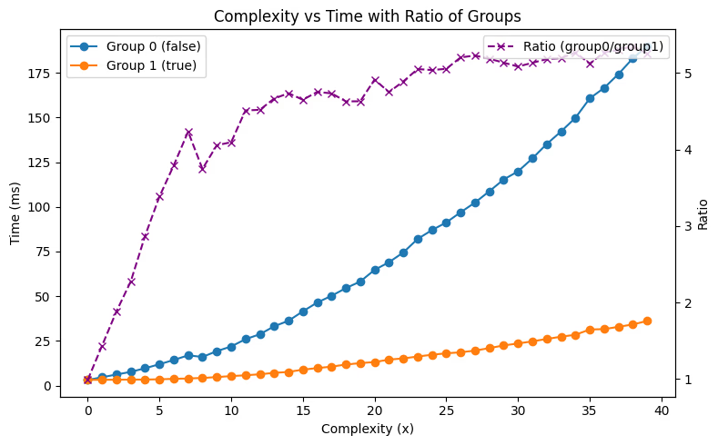
On x axis we have complexity parameter, on left y axis time in ms, and on right y axis ratio of times for SIMD to Fallback.
The most interesting observations:
- for
complexity=0SIMD is slightly slower than fallback due to SIMD overhead - for small
complexitySIMD is slightly faster than fallback and these ration grows - for higher
complexitySIMD is significantly faster but ratio stabilizes around5.2
If we would like to model time of computation as:
where is time fallback, is time simd, is time without complexity (mainly time of memory movement), and are coefficients describing cpu performance (lower is better), and is complexity parameter.
Then our theoretical ratio would look like:
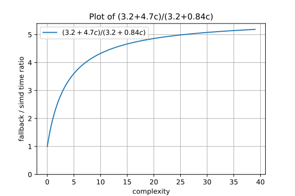
In SIMD we process 8 lines so naive intuition can suggest that , but in reality, it is not true due to SIMD overhead
There is a small overhead to:
- Packing/unpacking slices into f32x8 (from_slice and copy_to_slice)
- Handling leftover elements (the remainder loop)
- Loop control and alignment fixes
These operations are not free. For small workloads or low “complexity,” this overhead eats into the theoretical speedup.
Other articles
You can find interesting also.

Analysis of Zipf's Law in Node.js
Learn how to read large files in Node.js, count word occurrences using the Map object, and handle memory limits.
Daniel Gustaw
• 6 min read

CodinGame: Quaternion Multiplication - Rust, NodeJS - Parsing, Algebra
In this article, we will see how to implement the multiplication of quaternions in Rust and NodeJS. You will learn about parsing and algebra.
Daniel Gustaw
• 17 min read
Data Structuring on the Example of CHF NBP Course
Learn how to write code that normalizes and structures data based on a case study in the field of finance.
Daniel Gustaw
• 27 min read